The Social Insurance Code 58 Ch. 10 § (SFB) (2010:110) requires that the income index be calculated for each year. By Government decision, the Swedish Pensions Agency is to calculate and prepare proposals for an income index, which the Government then confirms. In addition, the Agency is required by the Regulations for the Earnings Related Old Age Pension (1998:1340) to calculate and confirm factors for inheritance gains, administrative costs and annuity divisors.
According to 64 Ch. 3 § SFB, premium pension operations are to be conducted according to sound insurance principles. These principles, as interpreted by the Swedish Pensions Agency, govern the calculation of the bonus rate, inheritance gains and annuity divisors for the premium pension. Further, the Swedish Pensions Agency is to calculate the fee that will finance premium pension operations.
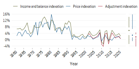
The change in the income index shows the development of the average income. Here, income refers to pension-qualifying income without limitation by the ceiling, but after deduction of the individual pension contribution.
\(\text{(A.1.1)}\quad\) \(\displaystyle I_t = I_{t-1} \cdot \frac{ u_{t-1} }{ u_{t-2} }\)
\(\text{(A.1.2)}\quad\) \(\displaystyle u_t = \frac{Y_t}{N_t}\)
- \(t\)
- calendar year
- \(I_t\)
- income index year \(t\)
- \(u_t\)
- average pension-qualifying income in year \(t\). The denominator uses the same income data previously used to calculate the income index for the previous year and is therefore an estimate.
- \(Y_t\)
- total pension-qualifying income without limitation by the ceiling, person aged 16–64 in year \(t\), after deduction of the individual pension contribution.
- \(N_t\)
- number of persons aged 16–64 with pension-qualifying income in year \(t\)
As of 2017, the income index is calculated according to new rules (SFS 2015: 676). The income index for year \(t\) will measure the change in average income between the years \(t-2\) and \(t-1\). Pension qualifying income is first known after taxation, that is, in December of the year following the income year. This means the income of the two most recent years is based on estimates. The income data used in the denominator is the same income data used for previous years. For 2018, the income index was calculated in a special way \(I_{t}=I_{t-2} \cdot u_{t-1}/u_{t-3}\). Income index for year \(t\) is thus corrected by the outcome for the year \(t-3\). In the denominator for this calculation year, the outcome of average pension-qualifying income is used.
When balancing is activated, the balance index is used instead of the income index.
\(\text{(A.2.1)}\quad\) \(\displaystyle B_{t} = I_t \cdot BT^{*}_t\)
\(\text{(A.2.2)}\quad\) \(\displaystyle B_{t+1} = B_t \cdot \biggl( \frac{ I_{t+1} }{ I_t }\biggr) \cdot BT^{*}_{t+1} = I_{t+1} \cdot BT^{*}_t \cdot BT^{*}_{t+1}\)
- \(B_t\)
- balance index year \(t\)
- \(I_t\)
- income index year \(t\)
- \(BT^{*}_t\)
- damped balance ratio year \(t\)1
At the turn of the year \((t-1) \to t\), indexation takes place via multiplication of pensions by the ratio between the balance index for year \(t\) and the income index for year \({t-1}\) divided by 1.016, and of pension balances by the ratio between the balance index for year \(t\) and the income index for year \({t-1}\). At the end of year \(t\), there is analogous indexation of the ratio between the balance index for year \(t+1\) and the balance index for year \(t\). Indexation by the balance index ceases when the balance index reaches the level of the income index.
In the premium pension system the amount to pay out is recalculated each year based on the value of the premium pension account. For those with fund insurance the yield from the account will depend on the fund returns, while for those with traditional insurance with profit annuity the value of the account will depend on the rate of return. The guaranteed amount in traditional insurance remains unchanged during the payout period, but it is increased if new premiums are received. The rate of return does not affect the amount of the life-insurance provisions since the pension liability is calculated on the basis of expected future payments of guaranteed amounts.
The pension balances of deceased persons are credited to the survivors in the same age group in the form of inheritance gains. For the economically active, this is done through multiplying the pension balances of the survivors by an annually calculated inheritance gain factor for the inkomstpension.
\(\text{(A.4.1)}\quad\) \(\displaystyle AF_{i, t} = \begin{cases} 1 + \frac{\sum\limits_{j=2}^{17} PBd_{j-1, t-1}}{\sum\limits_{j=2}^{17} PB_{j-1, t-1}}, & i = 2,3,...,17 \\ 1 + \frac{PBd_{i-1, t-1}}{PB_{i-1, t-1}}, & i = 18,19,...,60 \\ \frac{L_{i-1, t} + L_{i, t}}{L_{i, t} + L_{i+1, t}}, & i = 60,61,... \\ \end{cases}\)
- \(i\)
- age at end of year \(t\)
- \(AF_{i, t}\)
- inheritance gain factor \(t\) for age group \(i\)
- \(PBd_{i, t}\)
- pension balances of persons dying in year \(t\) in age group \(i\)
- \(PB_{i, t}\)
- total pension balances of survivors in year \(t\) in age group \(i\)
- \(L_{i, t}\)
- number of survivors in year \(t\) in age group \(i\) out of 100,000 born, according to the life span data of Statistics Sweden for the five-year period immediately preceding the year when the insured reaches age 60 for \(i\)= 60–64 and age 64 for \(i\)= 65 or older.
For persons 60 years of age or less, the inheritance gain factor is calculated as the sum of the pension balances of the deceased divided by the sum of the pension balances for the survivors in the same age group. For the group aged 2–17 years, a common inheritance gain factor is calculated. As there is some delay in information on persons dying during the year, the distribution of inheritance gains to persons aged 60 or less is made with a time lag of one year. For older persons, inheritance gain factors are calculated on the basis of the life-expectancy statistics from Statistics Sweden.
Inheritance gains arising after retirement are implicitly taken into account in the annuity divisor, through redistribution from individuals who die earlier to those who live longer. For the purpose of distributing inheritance gains by the same principle for both the economically active and retirees in the same birth cohort, the method of allocation is changed from age 60 on. By switching methods when the individual turns 60, the backlog in the distribution of inheritance gains before pension withdrawal. In the year when an insured turns 60, he or she is credited with double inheritance gains because of the two different procedures. In 2021, the change of method will take place at age 61 instead of 60 because the minimum withdrawal age has been raised to 62. Subject to a transitional provision, the age limit will be 60 in 2020.
The impact of inheritance gains on the pension liability is limited, for the pension balances of deceased persons are redistributed to the survivors. There is, however, an effect on the inkomstpension liability to the economically active because of the difference between inheritance gains arising and inheritance gains distributed; this effect is shown in Note 10, Chapter 8. For the group dying before their 60th year, the difference is explained by tax assessment changes between the time when inheritance gain factors are calculated and the time when the gains are distributed, and by late information on persons dying. For the group dying in their 60th year or thereafter, the reasons are differences between estimated and actual mortality, and possible variations in mortality depending on the insured’s level of income, i.e. the effect due to the shorter average life spans, for each gender, of persons with low incomes compared to persons with high incomes.
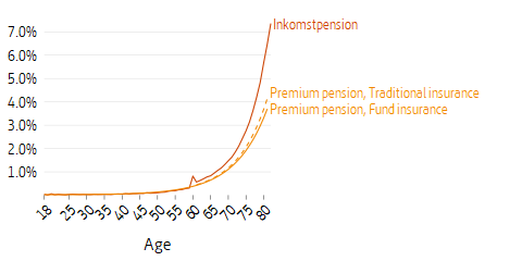
In the premium pension system, inheritance gains are calculated as a percentage of the premium pension capital of the survivors. The percentage corresponds to the one-year risk of death, i.e. the probability of dying within one year. Inheritance gains are distributed once a year for both the economically active and retirees. As with the inkomstpension, future expected inheritance gains are included in the annuity divisor. If the insured elects a survivor benefit, the inheritance gain will be much smaller, as it is then based on the probability that the longer-surviving party, whether the primary insured or the co-insured, will die within one year of the first party.
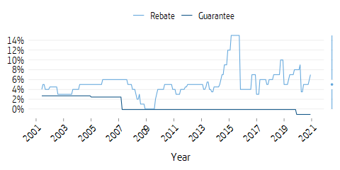
The risk of death in year \(t\) is calculated by Makeham’s formula (see Annuity Divisors for the premium pension). The values of \(a\), \(b\) and \(c\) in the formula are determined by the relationship between the capital of pension savers dying in year \(t-1\)and the capital of the surviving pension savers in the same year, calculated for each age group. The pension capital used to determine the inheritance gain in year \(t\) corresponds to the average balance of the premium pension account as of the last day of every month of year \(t-1\). The amounts of the inheritance gains are adjusted by a factor (close to 1) that will equalize with the greatest possible accuracy the total amount distributed in year \(t\) and the capital of pension savers dying in year \(t-1\).
The inheritance gains for the premium pension fund insurance do not affect the pension liability over time, as death capital is offset by inheritance gains distributed.
| a | b | c | factor | |
|---|---|---|---|---|
| Fund insurance | 0.00013 | 0.0000053 | 0.1091 | 0.9938 |
| Traditional insurance | 0.00070 | 0.0000027 | 0.1188 | 0.9905 |
The costs of administering the inkomstpension system reduce the pension balances of the economically active. The deduction from pension balances is recalculated annually through multiplication of pension balances by an administrative-cost factor.
\(\text{(A.6.1)}\quad\) \(\displaystyle FF_t = 1 - \biggl(\frac{B_t \cdot A_t + J_{t-1}}{PB_{t-1}}\biggr)\)
- \(FF_t\)
- administrative cost factor, year \(t\)
- \(B_t\)
- budgeted costs of administration, year \(t\)
- \(A_t\)
- proportion charged to pension balances, year \(t\)
- \(J_t\)
- adjustment amount, equals the difference between the amount that would have been deducted from pension balances in year \(t\), based on actual cost in year \(t\) and the adjustment amount in year \(t-1\), as well as the actual deduction taken from pension balances in year \(t\)
- \(PB_{t}\)
- total pension balances, year \(t\)
The administrative-cost factor is calculated on the basis of a certain proportion, \(A\), of budgeted costs for year \(t\). Until the year 2021, the proportion charged to pension balances will be less than 100 percent (see Note 11). Moreover, there is an adjustment for the administrative costs of year \(t-1\). The adjustment amount is equal to the difference between the amount that would have been deducted from pension balances, based on actual cost and the adjustment amount for the previous year, and the actual deduction made from pension balances in the same year.
The administrative-cost factor affects the inkomstpension liability to the economically active via the deduction from pension balances (see Note 14, Table 8.21 A in Chapter 8). The difference between total costs of administration (see Note 4 in chapter 8) and the deduction from pension balances puts a strain on the balance ratio.
In the premium pension a charge is deducted from pension savers’ premium pension accounts once a year. The charge is to cover the total operating costs of the premium pension, including interest and other financial expenses.
Administrative costs affect the capital of the premium pension system and at the same time, through the deduction from pension balances, they affect the premium pension liability by the same amount (see Note 17 and note 20) for fund insurance. For traditional insurance with profit annuity, life-insurance provisions are affected by assumptions of future expected operating costs.
The annuity divisors for the inkomstpension are used for recalculation of pension balances as annual disbursements and are a measure of life expectancy at retirement, with consideration given to the interest of 1.6 percent (advance interest) credited to pensions in advance.
\(\text{(A.8.1)}\quad\) \(\displaystyle D_i = \frac{1}{12L_i} \sum\limits_{k=i}^{r} \sum\limits_{X=0}^{11} \biggl( L_k + (L_{k+1} - L_k) \frac{X}{12} \biggr) (1.016)^{-(k-i)} (1.016)^{\frac{-X}{12}}, \quad i = 62, 63, ..., r\)
- \(D_i\)
- annuity divisor for age group \(i\)
- \(k-i\)
- number of years of retirement (\(k=i\), \(i+1\), \(i+2\), etc.)
- \(X\)
- number of months (0,1,…,11)
- \(L_i\)
- number of survivors in age group \(i\) per 100,000 born, according to the life span statistics of Statistics Sweden. These statistics are for the five-year period immediately preceding the year when the insured reached age 61 in the case of pension withdrawal before age 65, and age 64 in the case of withdrawal thereafter
For persons who have begun drawing their old-age pensions before age 65, the amount disbursed is recalculated, because of the recalculated annuity divisors, at the outset of the year when the individual turns 65. The reason for the recalculation is the change in the underlying statistical data for the latest life expectancy statistics available in the individual’s 65th year. With the continuing increase in life expectancy, the recalculated annuity divisors have so far been higher than before, resulting in reduction of future monthly pensions. The consequent marginal decrease in the inkomstpension liability to retirees is a component of the Change in Amounts Disbursed in Note 14, Table 8.21 C in Chapter 8.
After age 65, there is no further recalculation of annuity divisors. The increase in the pension liability of the system resulting from the fixed annuity divisors puts strain on the balance ratio when life expectancy is increasing.
Drawing an old-age pension involves a transfer of pension liability from the economically active to retirees. The actual recalculation of pension balances as annual disbursements results in a marginal change in the pension liability. The change arises because of the difference between annuity divisors and what we refer to as “economic annuity divisors” in this report. For a description of economic annuity divisors, see Appendix B Mathematical Description of the Balance Ratio, Pension Liability. The economic annuity divisors are used to calculate the pension liability to retirees.
Annuity divisors are determined for each age with no upper age limit.
| 61 | 62 | 63 | 64 | 65 | 66 | 67 | 68 | 69 | 70 | |
|---|---|---|---|---|---|---|---|---|---|---|
| 1938 | 17.87 | 17.29 | 16.71 | 16.13 | 15.56 | 14.99 | 14.42 | 13.84 | 13.27 | 12.71 |
| 1939 | 17.94 | 17.36 | 16.78 | 16.19 | 15.62 | 15.04 | 14.47 | 13.89 | 13.32 | 12.76 |
| 1940 | 18.02 | 17.44 | 16.86 | 16.27 | 15.69 | 15.11 | 14.54 | 13.96 | 13.39 | 12.82 |
| 1941 | 18.14 | 17.56 | 16.98 | 16.39 | 15.81 | 15.23 | 14.65 | 14.08 | 13.50 | 12.94 |
| 1942 | 18.23 | 17.65 | 17.06 | 16.48 | 15.89 | 15.31 | 14.74 | 14.16 | 13.59 | 13.02 |
| 1943 | 18.33 | 17.75 | 17.16 | 16.58 | 15.99 | 15.41 | 14.84 | 14.26 | 13.68 | 13.11 |
| 1944 | 18.44 | 17.86 | 17.28 | 16.70 | 16.11 | 15.54 | 14.96 | 14.38 | 13.80 | 13.23 |
| 1945 | 18.55 | 17.96 | 17.38 | 16.80 | 16.22 | 15.64 | 15.07 | 14.48 | 13.91 | 13.33 |
| 1946 | 18.64 | 18.05 | 17.47 | 16.89 | 16.31 | 15.73 | 15.16 | 14.57 | 13.99 | 13.41 |
| 1947 | 18.73 | 18.15 | 17.56 | 16.98 | 16.40 | 15.83 | 15.24 | 14.66 | 14.07 | 13.49 |
| 1948 | 18.83 | 18.24 | 17.66 | 17.07 | 16.49 | 15.91 | 15.33 | 14.74 | 14.16 | 13.58 |
| 1949 | 18.89 | 18.31 | 17.72 | 17.13 | 16.55 | 15.97 | 15.38 | 14.79 | 14.21 | 13.63 |
| 1950 | 18.98 | 18.39 | 17.80 | 17.21 | 16.63 | 16.05 | 15.46 | 14.87 | 14.28 | 13.70 |
| 1951 | 19.06 | 18.48 | 17.89 | 17.30 | 16.71 | 16.13 | 15.54 | 14.95 | 14.37 | 13.78 |
| 1952 | 19.14 | 18.55 | 17.96 | 17.37 | 16.78 | 16.20 | 15.61 | 15.02 | 14.43 | 13.85 |
| 1953 | 19.20 | 18.62 | 18.03 | 17.44 | 16.85 | 16.26 | 15.68 | 15.09 | 14.50 | 13.91 |
| 1954 | 19.28 | 18.69 | 18.11 | 17.52 | 16.93 | 16.34 | 15.76 | 15.17 | 14.58 | 13.99 |
| 1955 | 19.34 | 18.75 | 18.16 | 17.58 | 16.99 | 16.40 | 15.81 | 15.22 | 14.63 | 14.04 |
| 1956 | 19.42 | 18.84 | 18.25 | 17.66 | 17.07 | 16.48 | 15.89 | 15.30 | 14.71 | 14.12 |
- Annuity divisors are confirmed each year for all ages, but the table shows only the divisors up to age 70.
To calculate the annual premium pension, the value of the premium pension account is divided by an annuity divisor for the premium pension. Unlike the inkomstpension, the annuity divisor for the premium pension is based on forecasts of life expectancy.
\(\text{(A.9.1)}\quad\) \(\displaystyle D_x = \int\limits_{0}^{\infty} e^{-\delta t} \frac{l(x+t)}{l(x)} dt\)
\(\text{(A.9.2)}\quad\) \(\displaystyle \delta = ln(1+r) - \epsilon\)
\(\text{(A.9.3)}\quad\) \(\displaystyle l(x) = e^{-\int\limits_{0}^{x} (1-s) \mu(t) dt}\)
\(\text{(A.9.4)}\quad\) \(\displaystyle \mu(x) = \left\{ \begin{array}{l l} a + be^{cx} & \quad \text{when } x \leq 100\\ \mu(100) + (x-100) \cdot 0.01 & \quad \text{when } x > 100 \end{array} \right.\)
- \(D_x\)
- annuity divisors
- \(x\)
- exact age at time of calculation
- \(r\)
- interest rate
- \(\epsilon\)
- interest intensity of operating costs
- \(s\)
- mortality charge
The annuity divisors are calculated in continuous time and according to exact age at retirement, but in principle they are consistent with the formula for the annuity divisor for the inkomstpension.2 The survival function, \(l(x)\), can be considered equivalent to the number \(L\) used in the calculation of the inkomstpension. The mortality function, \(\mu(x)\), is the so-called Makeham’s formula used for calculating the risk of death within one year. The values of a, b and c correspond to Statistics Sweden’s forecast of remaining life expectancy in the years 2015–2110 for individuals born in 1938, 1945 or 1955.
So-called cohort mortality is used, which means that the year cohort 1938 is used for individuals born in the 1930s or earlier, year cohort 1945 is used for individuals born in the 1940s, and year cohort 1955 is used for individuals born in the 1950s or later. For x> 100 \(\mu(x)\) merges with a straight line with a slope of 0.01. During 2016, a charge \(s\) was imposed on mortality intensity following an analysis of how premium pension mortality differed from that found in Statistics Sweden.
| Cohort | a | b | c | s |
|---|---|---|---|---|
| 1930s | 0.00005 | 0.00000198 | 0.1239 | 0.1 |
| 1940s | 0.00460 | 0.00000053 | 0.1373 | 0.1 |
| 1950s | 0.00470 | 0.00000019 | 0.1476 | 0.1 |
When calculating the guaranteed amount in traditional insurance with profit annuity, the Statistics Sweden alternative with low mortality is used, reduced by a further 10 percent.
In the calculation of the payment amount, the interest rate assumption is called advance interest rate. The interest intensity \(\delta\) is based on the interest rate of 1.75 percent for both fund insurance and traditional insurance, reduced by the interest intensity for operating expenses of 0.1 percent, which corresponds to \(\delta\)= 0.016349.
When calculating the annuity divisor to produce the guaranteed amount in the traditional insurance, we use Statistics Sweden’s alternative with low mortality reduced by a further 10 percent, an interest rate which is -1.0 percent and an interest intensity for operating expenses of 0.1 percent.
In traditional insurance, the technical insurance provision, FTA (“pension liability“), consists of life insurance provision, unpaid claims and other technical insurance provisions. The life insurance provision is determined for each insurance as the capital value of remaining guaranteed payments. The value is calculated using assumptions about the discount rate, mortality and operating costs. As of May 1, 2017, when a new law regulating the Swedish Pensions Agency’s premium pension operation came into effect, the discount rate is given by an interest rate curve that is the average of the interest rate curve for government bonds and mortgage bonds. The mortality assumption is different for men and women, but otherwise calculated as for amounts to be paid out, cohort-based and using Statistics Sweden’s forecast with a deduction of 10 percent. Operating expenses are assumed to be 0.07 percent of the capital.
Unpaid claims are pension disbursements that have not been able to be carried out. Remaining technical provisions consist of reductions from the transfer of pension credit between spouses not yet distributed. These two items are very small compared to the life insurance provision.
| 61 | 62 | 63 | 64 | 65 | ||
|---|---|---|---|---|---|---|
| Without survivor benefit | 20.91 | 20.37 | 19.82 | 19.26 | 18.69 | |
| With survivor benefit | Co-insured 55 | 26.30 | 26.12 | 25.95 | 25.80 | 25.65 |
| Co-insured 60 | 24.69 | 24.44 | 24.19 | 23.96 | 23.75 | |
| Co-insured 65 | 23.39 | 23.05 | 22.72 | 22.40 | 22.10 | |
| Co-insured 70 | 22.31 | 21.88 | 21.45 | 21.04 | 20.63 | |
| 66 | 67 | 68 | 69 | 70 | ||
| Without survivor benefit | 18.12 | 17.54 | 16.29 | 15.71 | 15.13 | |
| With survivor benefit | Co-insured 55 | 25.51 | 25.38 | 25.17 | 25.06 | 24.97 |
| Co-insured 60 | 23.55 | 23.36 | 23.04 | 22.89 | 22.75 | |
| Co-insured 65 | 21.81 | 21.53 | 21.06 | 20.83 | 20.63 | |
| Co-insured 70 | 20.23 | 19.84 | 19.12 | 18.79 | 18.47 | |
| 61 | 62 | 63 | 64 | 65 | ||
|---|---|---|---|---|---|---|
| Without survivor benefit | 32.49 | 31.38 | 30.27 | 29.17 | 28.09 | |
| With survivor benefit | Co-insured 55 | 44.62 | 44.18 | 43.76 | 43.38 | 43.02 |
| Co-insured 60 | 40.58 | 39.97 | 39.40 | 38.88 | 38.39 | |
| Co-insured 65 | 37.57 | 36.78 | 36.04 | 35.34 | 34.68 | |
| Co-insured 70 | 35.52 | 34.59 | 33.70 | 32.84 | 32.01 | |
| 66 | 67 | 68 | 69 | 70 | ||
| Without survivor benefit | 27.01 | 25.94 | 24.89 | 23.84 | 22.81 | |
| With survivor benefit | Co-insured 55 | 42.70 | 42.40 | 42.12 | 41.87 | 41.63 |
| Co-insured 60 | 37.94 | 37.53 | 37.15 | 36.80 | 36.48 | |
| Co-insured 65 | 34.06 | 33.49 | 32.95 | 32.46 | 32.01 | |
| Co-insured 70 | 31.22 | 30.47 | 29.77 | 29.10 | 28.48 | |
In chapter 6 Changes in the Value of the Pension System, two different measures are used for calculating the change in value in the premium pension system. These measures are time-weighted return and capital-weighted return. They are briefly described below.
The capital-weighted rate of return takes into consideration the capital flow of the account by weighing together the return and the capital in the account during the corresponding period. This means that during periods when the sum under capital management has been large, the return is given greater weight in the calculation than the return during periods when there has been little capital managed. The cash flows chiefly included in the calculations consist of paid-in pension credit and pension disbursements. The interest on the preliminary pension credit, the return on the funds in the portfolio, the administration fee to the Swedish Pensions Agency, the management fee to fund companies, the bonus on the management fee and inheritance gains are not included in the cash flows, but affect the return directly.
When the capital-weighted return is calculated, the so-called internal rate of return is sought. This rate is a discount rate at which the present value of all cash flows, including the value of the closing balance but with the opposite sign, will equal zero.
The capital-weighted return (also referred to as the Internal Rate of Return, or IRR) is calculated by solving the equation
\(\text{(A.10.1)}\quad\) \(\displaystyle \sum_{t=0}^{T} \frac{C_t}{(1 + r)^{\frac{t}{365}}} = 0\)
- \(r\)
- internal rate of return during the period, expressed as an annual rate
- \(t\)
- number of days since the starting point
- \(T\)
- closing point
- \(C_t\)
- transaction (cash flow) at time \(t\)
- \(C_T\)
- final value, that is, the value of the account as of the day when the valuation is made
The equation requires that the final value be negative so that a value of SEK \(X\) results in a transaction of SEK \(-X\). \(C_T\) is thus always \(\le\) 0.
To calculate the internal rate of return, it is therefore necessary to know the closing value of the portfolio (market value), all cash flows to and from the portfolio, and the time when these cash flows take place. The internal rate of return can be said to yield the “interest rate on bank accounts” which, given the deposits and withdrawals, have resulted in the current closing value.
The formula above for the internal rate of return is the one normally used in financial matters.
It can also be expressed in the following way, which is consistent with how interest is actually credited to bank accounts:
\(\text{(A.10.2)}\quad\) \(\displaystyle \sum_{t=0}^{T-1} C_t \cdot (1 + r)^{\frac{T-t}{365}} = C_T\)
Interest is earned on each deposit \(C_t\) from the time of deposit \(t\) until the closing date \(T\).
\(C_T\) is greater than or equal to zero, and is the balance at the time of calculation.
With the time-weighted return, adjustment is made for the effects of capital inflows and outflows, that is, to prevent new pension credit recorded or pensions paid from affecting the calculated rate of return. The time-weighted return thus measures the return for a certain deposited amount for a certain period of time. If time-weighted, the return is measured for a period, the returns for the partial periods are weighed together with equal weights. A partial period consists of the time between two cash flows. The equation below describes the time-weighted return.
\(\text{(A.10.3)}\quad\) \(\displaystyle R_t = \biggl(\prod_{t=0}^{T} \frac{MV_{t+1}}{MV_t + C_t}\biggr) - 1\)
- \(R_t\)
- return during the period
- \(t\)
- number of days since the starting point
- \(T\)
- closing point
- \(MV_t\)
- market value at time \(t\)
- \(C_t\)
- transaction (cash flow) at time \(t\)
The time-weighted return can be used to obtain accurate comparisons of the return between funds, where fund managers cannot set aside more capital under favourable return conditions or vice versa. The measure can also be used for comparisons with relevant market indices or with the return achieved by other managers. In the premium pension system, the pension saver cannot freely determine the in- or outflow of capital for the premium pension account. On the other hand, the saver decides whether and when the moneys invested are to be transferred to another fund. The fund companies have no influence over the flow of capital in the fund.
| How well are the funds doing? |
| – Time Weighted Return (Premium Pension Index) |
| How well are the pension savers doing? |
| – Capital-Weighted Return |
| How well are my funds doing? |
| – Time Weighted Return per Fund |
| – Time-Weighted Return for the Fund Portfolio |
| How well is my account/my pension doing? |
| – Capital-Weighted Return |